


You can trade Nvidia stock at 3am on a Sunday, through its perpetual future on Hyperliquid, while the underlying market on NASDAQ is closed. What does price discovery look like during the overnight session? What is driving price movements?
While Nasdaq is open, it anchors the price of these stocks, and arbitrageurs keep the perpetual futures in line. But nights, weekends and holidays add up to more than half the week. In those hours the perpetuals essentially run independent price discovery, influenced by the current market microstructure, potentially more than during peak liquidity.
We tested four simple signals, measuring how well each one predicts the next 15 minutes, segmenting into 2 different periods: while Nasdaq is open and then while it is closed. During regular hours, predictability is both low, but once Nasdaq closes, market microstructure metrics multiply their predictive power. We built a small model te demonstrate it: it made money out of sample when Nasdaq was closed and lost money when it was open, with the same features, fees and code.
Caveat: the edge is small and it is shrinking. It also needs fees under a basis point.
I. Overnight price discovery
trade.xyz is a stock-perp exchange built on Hyperliquid. It lists single names such as NVDA and TSLA, and two indices, SP500 and XYZ100 (its Nasdaq-100). Binance lists perps on 26 of the same names.
Every perpetual has a matching oracle feed. That is the reference price the exchange uses to mark positions and set funding. During regular hours it follows the price set by “tradFi” exchanges. What happens when that feed is inactive? Our hypothesis was that market microstructure metrics are considerably more predictive during these times.
To test it, I labelled every five-minute bar with its New York session. Overnight (20:00 to 04:00), weekends (Friday 20:00 to Sunday 20:00) and NYSE holidays count as closed. Regular hours (09:30 to 16:00) are the control. I left out the grey-zone: pre-market and after-hours, because some cash trading happens then. The data covers 28 of the most liquid US stock perps on trade.xyz, from January 1 to November 11, 2026. I pulled it with the Aperiodic Python client: l1_price for the best bid and ask and their sizes, and derivative_price for the oracle.
II. The microstructure metrics
Four metrics that we found to be predictive:
book imbalance: (bid size − ask size) / (bid size + ask size) at the best quotes;
the premium: how far the perp’s mid sits from the oracle, minus its 1-day average;
the perp’s own return over the last 15 minutes;
the
XYZ100index perp’s return over the last 15 minutes.
For each metric I computed its rank correlation (IC) with the next 15-minute mid return. I did this per symbol and then averaged across the 28. The t-statistics in brackets run across symbols. They show whether the effect holds name by name, not just in one name.
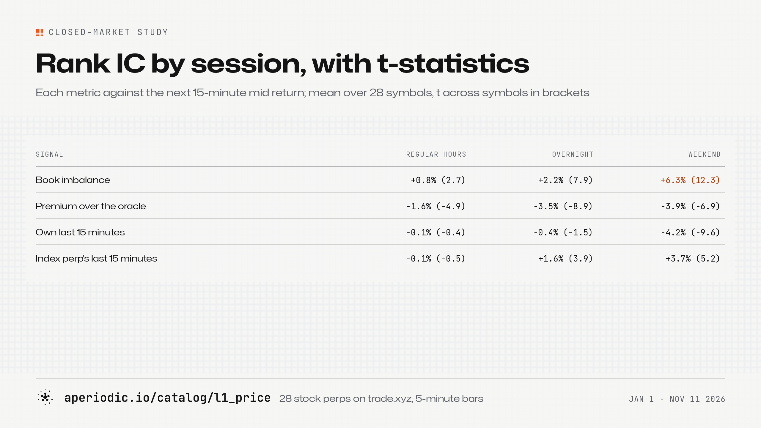
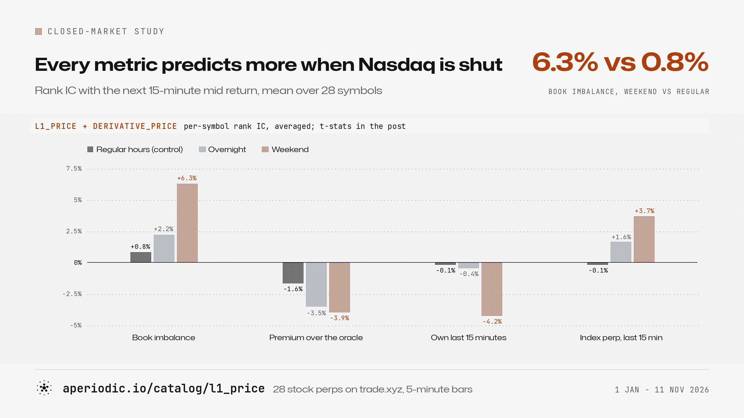
Every signal gets stronger from left to right. During regular hours the best one stays under 2%, and two are no different from zero. At weekends all four sit between roughly 4% and 6%, and every one is clearly significant.
Binance shows very similar results, with an additional predictive metric: the gap between Binance’s price and Hyperliquid’s. When Nasdaq is closed, Binance follows the price on Hyperliquid, and the gap predicts Binance’s next 15 minutes clearly (an IC of about −3%). During regular hours the gap, it loses all of its predictive power, which makes sense if both venues simply follow Nasdaq then.
One note on method. I measured every return from the mid price, never from the last trade, as those bounce between bid and ask, which disguises itself as a reversal that’s not actually tradeable. This is even more prominent during the illiquid weekend / overnight sessions.
III. The why
Let’s start with book imbalance: when Nasdaq closes it’s book is pretty thin: about $1,000 at the best quote. A lopsided queue on a book that thin usually moves the price the way it leans. There is little on the other side to stop it.
The premium and the reversal are one story seen from two ends. Someone sends a burst of orders in one direction. On a thin book, the price moves further than the news behind those orders justifies. The perp drifts away from its oracle, and part of the move comes back. Equity researchers call this the return to liquidity provision (Nagel 2012). It should be more predictive during times when market makers are lessa active.
The index lead is the familiar lead-lag between a liquid index and thinner single names. The XYZ100 perp moves first, and single names follow within minutes. My best guess is that people trade macro views through the index, so news reaches it before it reaches NVDA’s thin book. During the day the cash market and its futures take in news together, and the lag disappears.
Every metrics’ IC are also stronger at weekends than overnight. I think one reason covers all four. On weekday nights, Nasdaq-100 futures still trade in Chicago (CME’s hours), so the perps have a partial anchor, while not on the weekends.
IV. The model
We built an replicable, simple ensemble model with best practices to see if these low-capacity edges could be tradeable when combined.
We used 5 minute data as an input, with a potentiall important difference: the bars that do not see new quotes are nulled out, so a stale oder book imbalance is not carried forward. Every feature uses only data up to the end of its own bar, and is using local timestamped event aggregates that we serve at Aperiodic.
book_imbalance: (bid size − ask size) / (bid size + ask size), at the bar’s last best bid and askpremium: 10,000 × ln(mid / oracle), minus its own rolling mean over the last 288 bars (one day), per symbol, once at least 50 bars existreturn_15m: 10,000 × (ln mid now − ln mid three bars ago)index_return_15m:return_15mof theXYZ100perp at the same timestamptarget: 10,000 × (ln mid three bars ahead − ln mid now), clipped at ±300 bp
For each test month from April to November, I fit a new model on all previous bars of the same session group. The main model learns from closed bars (overnight, weekend, holiday), and the control learns from regular-hours bars. The window expands from January 1, so the training set grows from about 130,000 bars for the April refit to about 900,000 for November.
All 28 symbols share one model, and the model gets no symbol identifier. I drop training rows without a quote or a target. The training data stops two days before the test month starts, so no 15-minute target reaches into the test month. There is no early stopping, no validation split, and no tuning on the test months; I ran the grid in section VII after I had fixed the design.
The learner
The learner is LightGBM regressor, with the default hyperparameters, except:
Objective: Huber, with δ = 30 bp
Leaves per tree: 7
Minimum bars per leaf: 2,000
Learning rate: 0.05
Trees: 150, a fixed number
Seed: 1, deterministic mode
I chose Huber because 15-minute returns on these books have fat tails, and a squared loss lets a few big moves pull the whole fit. I kept the trees small and the leaves large so each split needs a broad pattern across thousands of bars.
What it learned
Out of sample, the closed-market forecast has a rank IC of 5.2% over about 820,000 test bars. The regular-hours model scores −0.3% over about 290,000. These two numbers pool every symbol and bar into one rank correlation; the single-signal table in section II averages per-symbol ICs instead.
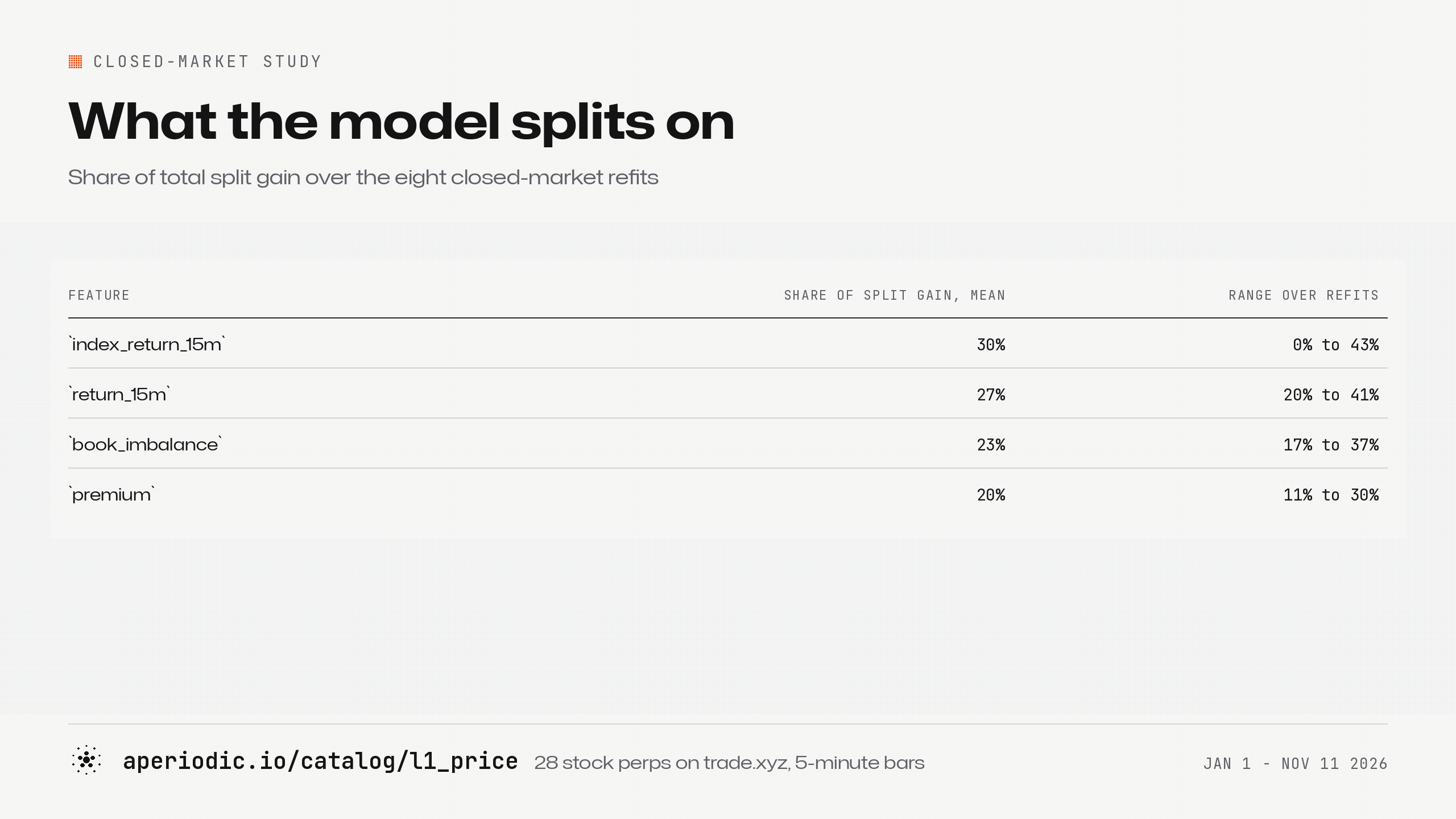
The four features, Averaged over the eight closed-market refits, each takes between a fifth and a third of the total split gain:
V. A follow-up test: Seoul and Tokyo
If the effect comes from the cash market being closed, it should follow each stock’s own exchange, not New York’s. trade.xyz lists three stocks that let us check this: SK Hynix, Samsung and Kioxia. They trade in Seoul and Tokyo, which are open during the US night.
I ran the same monthly refits, trained only on the US names’ closed bars, and applied each month’s model to these three. The model never saw them in training. On weekdays when both their home market and New York were closed, its IC was about 10%. At weekends it was about 6%. While Seoul and Tokyo were trading, it fell to 2%. And when New York was open but Seoul and Tokyo were not, it stayed around 6%. It makes sense: New York opening does nothing to anchor a stock that trades in Seoul or Tokyo.
Two caveats, thought: the weekend number is lower than the weekday one, the opposite of the US pattern, and I can’t explain that yet. I also used 00:00 to 06:30 UTC on weekdays as their home hours and ignored Korean and Japanese holidays, so the split is a little blurred.
It’s good sign for the original hypothesis that the model never saw these stocks, and it found its edge when their own exchanges were closed.
VI. Can you trade it?
The rule
At the close of every bar:
If no position is open, the absolute forecast is above the month’s threshold, and the spread is under 5 bp, enter in the forecast’s direction. A buy pays that bar’s last ask; a sell gets its last bid.
Fifteen minutes (three bars) later, check the forecast again. If it still points the same way and is above half the threshold, hold for another 15 minutes. Repeat, for at most 6 hours.
Otherwise exit across the spread: a long sells at the bid, a short buys back at the ask.
If bars are missing between entry and exit, skip the trade.
Charge 1.5 bp in fees on each side, on top of the spread.
The threshold is the 99.9th percentile of the absolute forecasts the model made on its own training data. Each refit sets its own: about 6 bp in April, and between 8 and 9.5 bp from June on (the monthly table below). Every trade has the same notional, and its result is its net return in bp.
Results
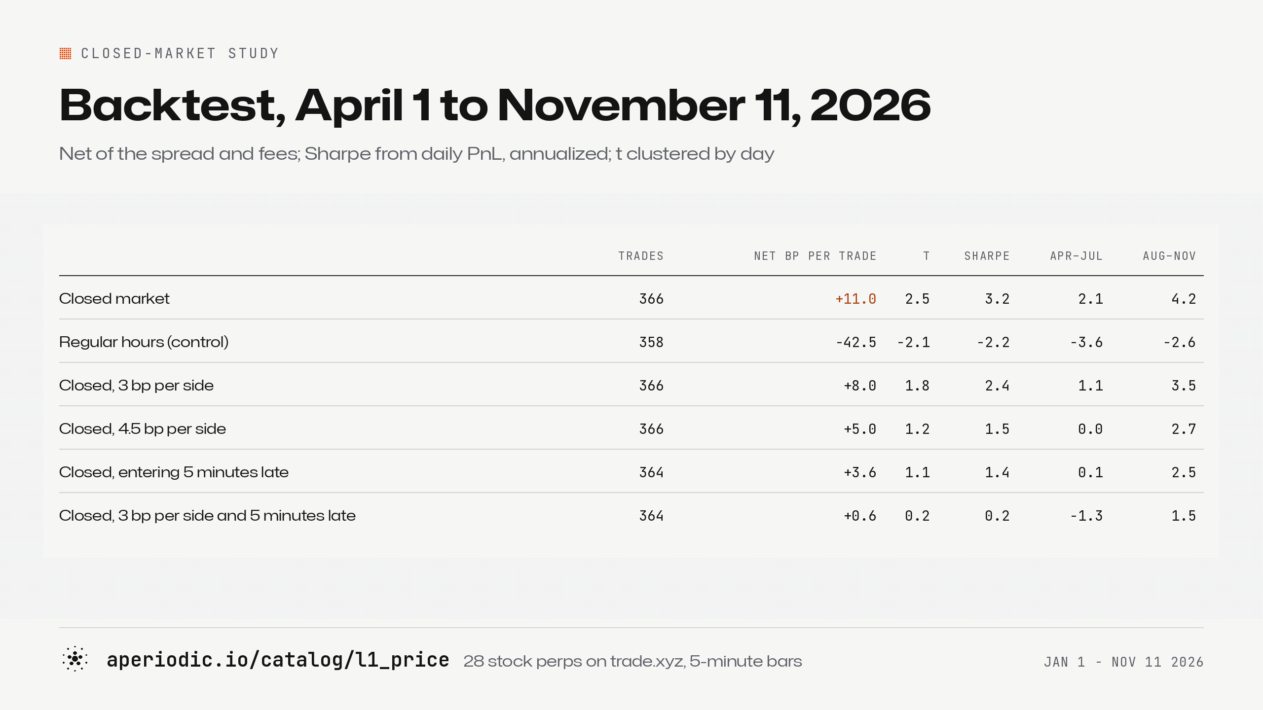
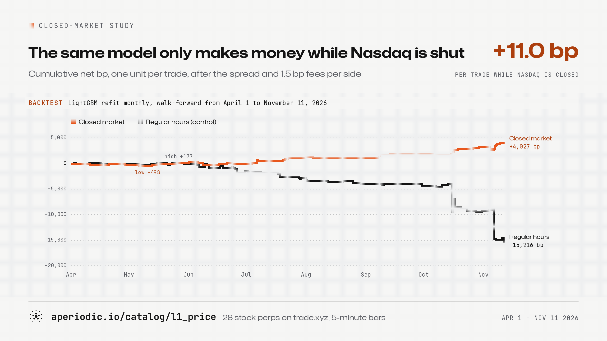
The base case makes about 11 bp a trade. Higher fees and a delay each take a large bite, and both together leave nothing.
Overnight: trades 175, net bp per trade +7.1
Weekend: trades 172, net bp per trade +12.1
Holiday: trades 19, net bp per trade +36.3
The trades
Trades: 366
Days with a trade: 126
Symbols traded: 27 of 28
Win rate: 57%
Longs: 342, +10.2 bp each
Shorts: 24, +22.1 bp each
Median holding time: 15 minutes
Trades held past 15 minutes: 9%
Trades that reached the 6-hour cap: none
Median spread at entry: 2.0 bp
Median absolute forecast at entry: 8.8 bp
The trades are highly skewed towads buy. The average long enters after the perp has fallen about 100 bp in 15 minutes. At that point it sits about 60 bp below its usual premium to the oracle, and the book leans toward the bid. The average short is the mirror image, after a rise of about 130 bp. So in practice the model mostly buys sharp drops that overshoot.
Could the long bias distort the results? Over all closed-market test “bars”, the average 15-minute return is about +0.1 bp, and it is positive exactly half the time. Drift explains almost none of the 10 bp per long edge. It’s difficult to tell exactly why the extreme forecasts are nearly all buys, but our guess is that sharp drops on a thin book overshoot more often than sharp spikes, and that’s the fundamental behaviour this model is trying to exploit.
Month by month
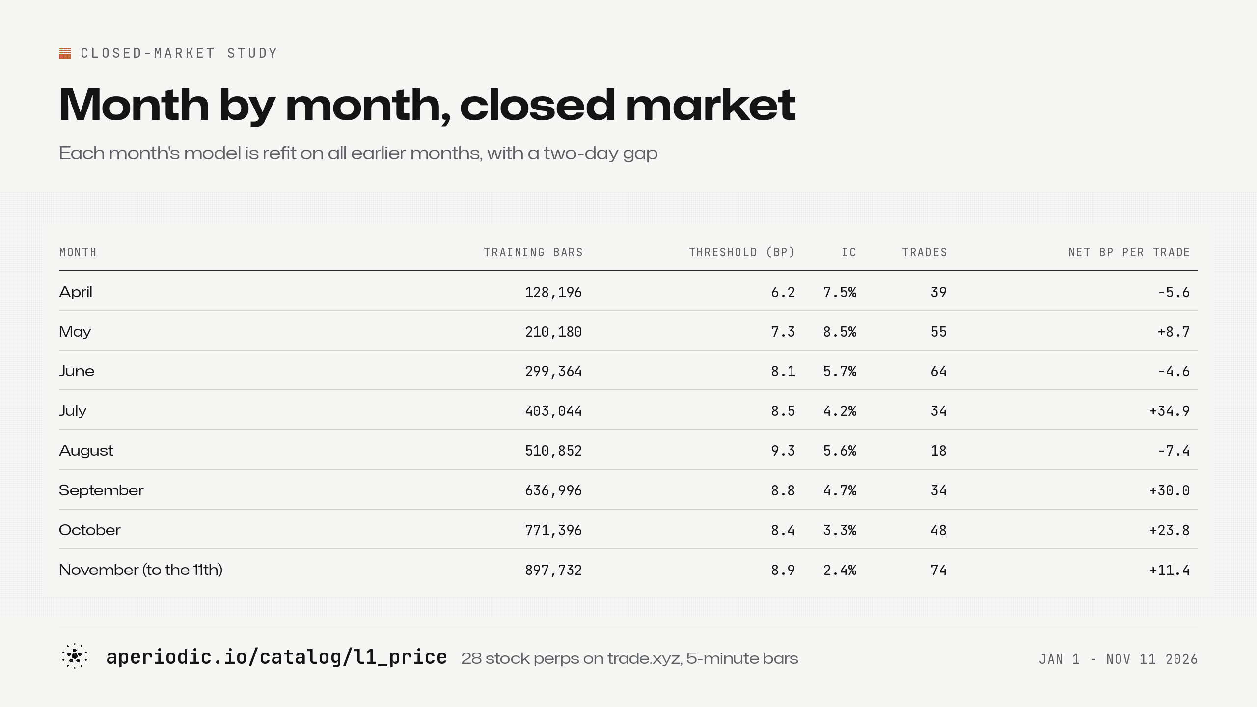
The IC falls in most months, from 8.5% in May to 2.4% in November, and three months lost money. See section VIII expanding on that.
The regular-hours control lost money in seven of its eight months, and its monthly IC never went above about 2%. Most of its losses came on three sell-off days in October and November. On each of them it bought many names at once and “held on”.
VII. How simpler and more complex model variations performed
A linear model ranks almost as well, but it doesn’t hit the original trading threshold. Plain OLS (an intercept and the four features, fit on rows with no missing values, with missing test values set to zero) reaches an IC of almost 5%. At a fixed 6 bp entry threshold it takes nearly 1,600 trades and makes less than 1 bp on each.
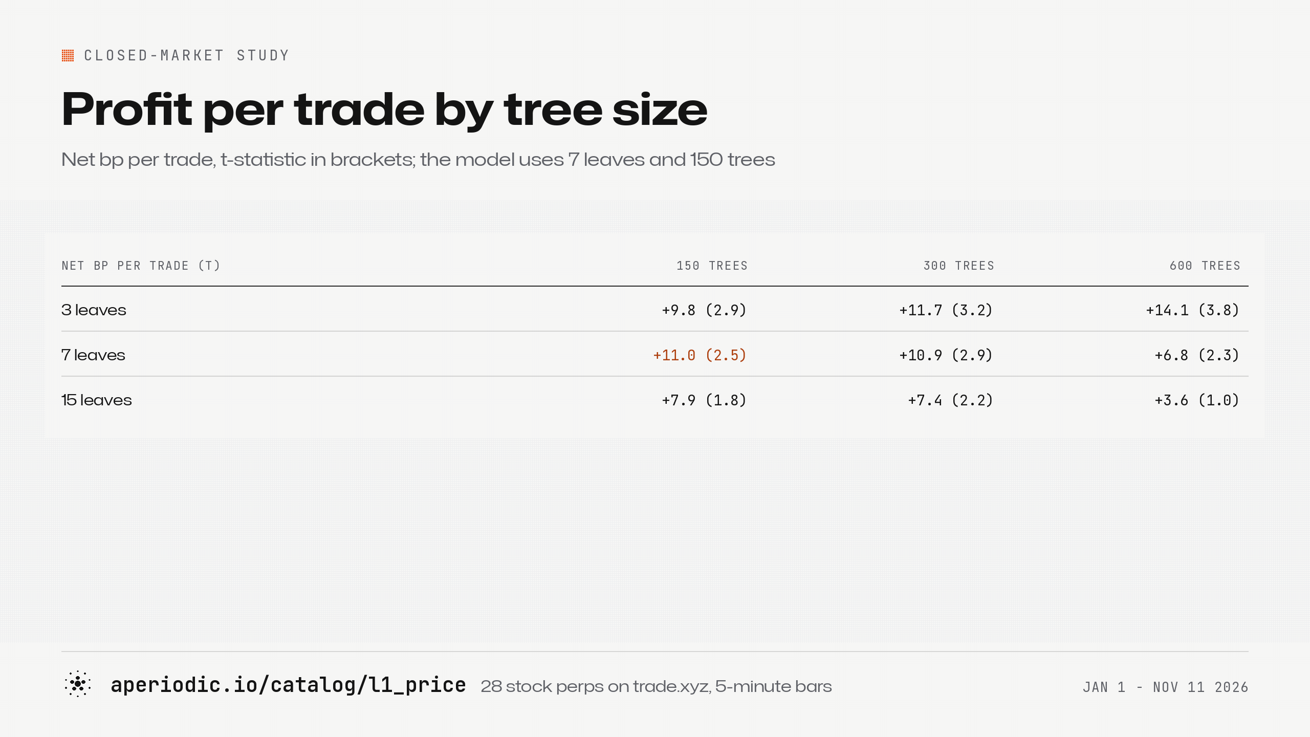
Deeper trees did worse. With 300 or 600 trees, profit per trade fell as the trees got deeper. More trees on shallow 3-leaf trees went the other way. But I ran this grid after choosing 7 leaves and 150 trees, so I wouldn’t swap in the better number.
The entry rule mattered less than I expected. I kept the 0.1% rate from an earlier version of this study. Rerun on the public data, April to July alone would have picked 0.2%:
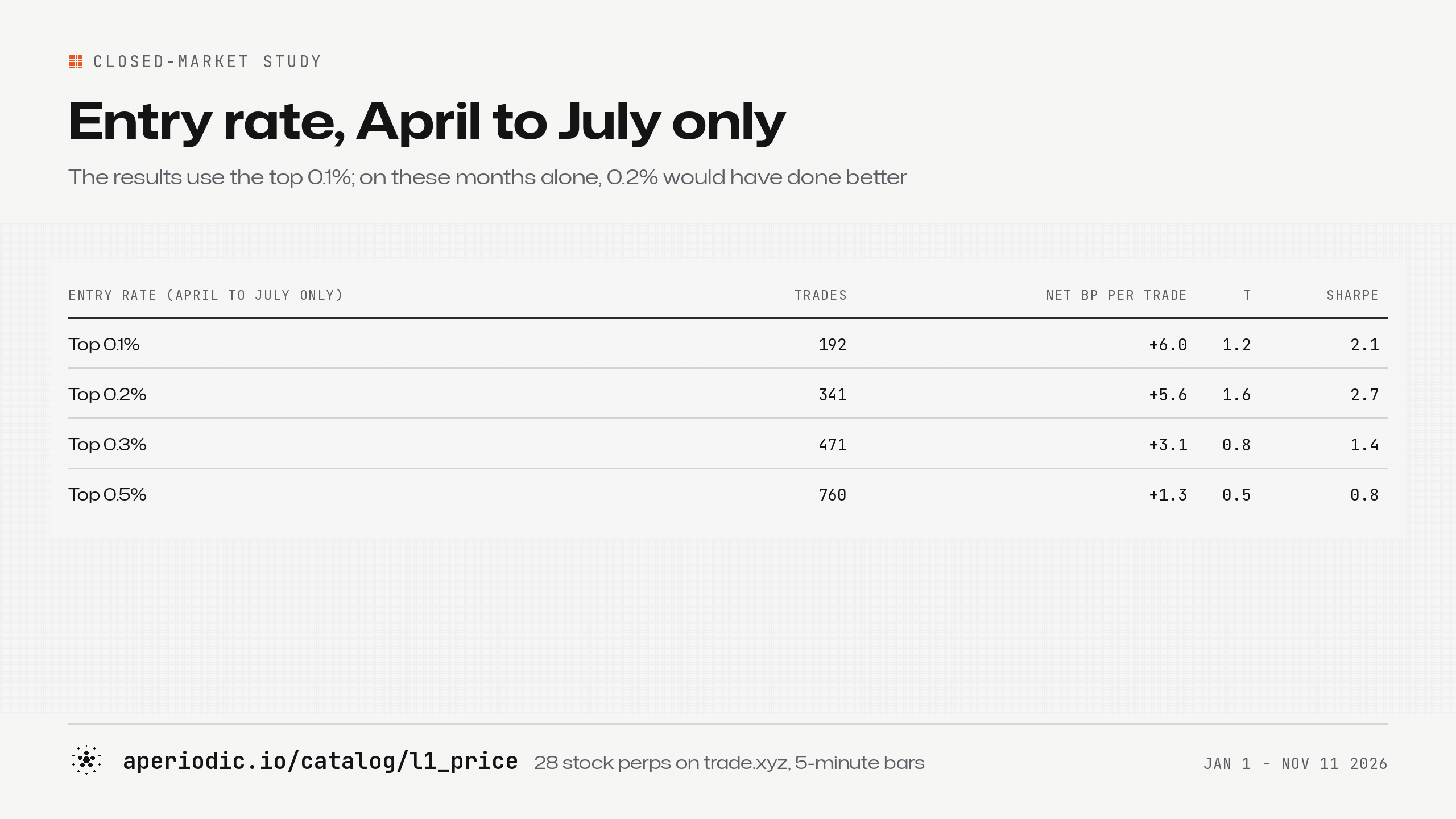
A fixed 8 bp threshold over the whole test period gave 469 trades at +9.8 bp each and the same Sharpe of 3.2 as the 0.1% rate.
VIII. Caveats
The edge is shrinking. The forecast’s IC was about 8% in April and May and below 2.5% in early November. Three of the eight months lost money. The obvious explanation is that others found these edges, and that liquidity is increasing.
It’s somewhat latency sensitive. Entering five minutes late cuts the profit from 11 bp a trade to under 4, and the t-statistic falls to about 1. The signals go stale within minutes.
It’s Fees decide whether it works at all. At 4.5 bp per side the profit drops to about 5 bp a trade. Hyperliquid’s docs put the taker fee on a HIP-3 market in growth mode at 0.0045% to 0.009%, under 1 bp, against 0.045% on the base perp tier (fees).
It is capacity-constrained: about $1,000 of top-level liquidity in the order book for a typical closed-hours bar.
It has a very significant long bias.
The backtest is too optimistic. Every trade is executed at the last bid and ask of its 5-minute bar, with no latency and no funding.
And the sample is short: seven and a half months, on a young exchange.
IX. Reproduce it
The one-signal version takes a minute. This pulls NVDA’s perp through the Aperiodic API and compares book imbalance on weekdays and weekends:
from datetime import date
import polars as pl
from aperiodic import get_metrics

q = get_metrics(metric="l1_price", timestamp="true", interval="5m",
                exchange="hyperliquid-perps", symbol="perpetual-XYZ:NVDA-USDC:USDC",
                start_date=date(2026, 9, 1), end_date=date(2026, 10, 31))

et = pl.col("time").dt.replace_time_zone("UTC").dt.convert_time_zone("America/New_York")
mid = ((pl.col("bid_price") + pl.col("ask_price")) / 2).log()
print(q.with_columns(
        imbalance=(pl.col("bid_amount") - pl.col("ask_amount")) / (pl.col("bid_amount") + pl.col("ask_amount")),
        next_15m=(mid.shift(-3) - mid) * 1e4,
        weekend=(et.dt.weekday() >= 6),
    )
    .group_by("weekend")
    .agg(ic=pl.corr(pl.col("imbalance").rank(), pl.col("next_15m").rank())))
For September and October it prints an IC of about 1% on weekdays and almost 4% at weekends.
The full study is a few short Python files on the same client, in aperiodic-io/notebooks:
data.pypulls the quotes and oracle prices and builds the 5-minute panel;model.pyholds the session calendar, the features, the refits and the backtest;study.pycomputes every table and both charts;details.pycomputes the refit, feature and trade details in sections IV and VI.
Run pip install "aperiodic[polars]" lightgbm, then python study.py --root ./closed_market.
Both the snippet and the full study need 2026 data, which comes with Pro. A free key gets you every metric for 2025 on BTC, ETH, SOL and 10 tokenized assets.. The metrics are l1_price and derivative_price.
Next I want to run the same test on other markets that trade around the clock against one that doesn’t: gold, oil and FX perps at the weekend. If you need help with data, feel free to DM me!
Appendix: universe and calendar
The 28 perps on trade.xyz, by the month of their first quote in our data:
January 2026: HOOD, INTC, MU, PLTR, TSLA
February: AAPL, COIN, CRCL, MSFT, ORCL
March: AMD, MSTR, NVDA
April: AMZN, GOOGL, META, SNDK,
XYZ100May: CRWV
June: RKLB,
SP500July: CBRS, MRVL
August: LITE, MRNA, NBIS, SOXL, SPCX
I label sessions in New York time, so they follow the daylight-saving switches. The NYSE full-day holidays in the calendar are January 1, January 19, February 16, April 3, May 25, June 19, July 3 and September 7 (November 26 falls after the sample ends).
References
Nagel, S. (2012). Evaporating liquidity. Review of Financial Studies, 25(7).